This Jupyter notebook can be downloaded from noise-fitting-example.ipynb, or viewed as a python script at noise-fitting-example.py.
PINT Noise Fitting Examples
[1]:
from pint.models import get_model
from pint.simulation import make_fake_toas_uniform
from pint.logging import setup as setup_log
from pint.fitter import Fitter

import numpy as np
from io import StringIO
from astropy import units as u
from matplotlib import pyplot as plt
[2]:
setup_log(level="WARNING")
[2]:
1
Fitting for EFAC and EQUAD
[3]:
# Let us begin by simulating a dataset with an EFAC and an EQUAD.
# Note that the EFAC and the EQUAD are set as fit parameters ("1").
par = """
    PSR             TEST1
    RAJ             05:00:00    1
    DECJ            15:00:00    1
    PEPOCH          55000
    F0              100         1
    F1              -1e-15      1
    EFAC tel gbt    1.3         1
    EQUAD tel gbt   1.1         1
    TZRMJD          55000
    TZRFRQ          1400
    TZRSITE         gbt
    EPHEM           DE440
    CLOCK           TT(BIPM2019)
    UNITS           TDB
"""

m = get_model(StringIO(par))

ntoas = 200

# EFAC and EQUAD cannot be measured separately if all TOA uncertainties
# are the same. So we must set a different toa uncertainty for each TOA.
# This is how it is in real datasets anyway.
toaerrs = np.random.uniform(0.5, 2, ntoas) * u.us

t = make_fake_toas_uniform(
    startMJD=54000,
    endMJD=56000,
    ntoas=ntoas,
    model=m,
    obs="gbt",
    error=toaerrs,
    add_noise=True,
    include_bipm=True,
)
[4]:
# Now create the fitter. The `Fitter.auto()` function creates a
# Downhill fitter. Noise parameter fitting is only available in
# Downhill fitters.
ftr = Fitter.auto(t, m)
[5]:
# Now do the fitting.
ftr.fit_toas()
[6]:
# Print the post-fit model. We can see that the EFAC and EQUAD have been
# and the uncertainties are listed.
print(ftr.model)
# Created: 2026-05-29T16:46:00.744887
# PINT_version: 1.1.5+106.g7d0f1d8
# User: docs
# Host: build-32906959-project-85767-nanograv-pint
# OS: Linux-7.0.0-1004-aws-x86_64-with-glibc2.35
# Python: 3.11.14 (main, Apr 27 2026, 17:28:30) [GCC 11.4.0]
# Format: pint
# read_time: 2026-05-29T16:45:57.967880
# allow_tcb: False
# convert_tcb: False
# allow_T2: False
PSR                                 TEST1
EPHEM                               DE440
CLOCK                        TT(BIPM2019)
UNITS                                 TDB
START              53999.9999999862564353
FINISH             56000.0000000056284375
DILATEFREQ                              N
DMDATA                                  N
NTOA                                  200
CHI2                   199.97653631096483
CHI2R                  1.0361478565334965
TRES                 1.858548914601668364
RAJ                      4:59:59.99999319 1 0.00000668346613640220
DECJ                    15:00:00.00127020 1 0.00058098663367164188
PMRA                                  0.0
PMDEC                                 0.0
PX                                    0.0
F0                   99.99999999999984669 1 2.6653297796922754106e-13
F1              -1.0000187187087043596e-15 1 1.1954074522964854619e-20
PEPOCH             55000.0000000000000000
PLANET_SHAPIRO                          N
TZRMJD             55000.0000000000000000
TZRSITE                               gbt
TZRFRQ                             1400.0
EFAC            tel gbt        1.6806468427815466 1 0.1569126783780669
EQUAD           tel gbt        0.3909754318140872 1 0.2466517758113335
[7]:
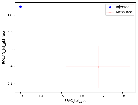
# Let us plot the injected and measured noise parameters together to
# compare them.
plt.scatter(m.EFAC1.value, m.EQUAD1.value, label="Injected", marker="o", color="blue")
plt.errorbar(
    ftr.model.EFAC1.value,
    ftr.model.EQUAD1.value,
    xerr=ftr.model.EFAC1.uncertainty_value,
    yerr=ftr.model.EQUAD1.uncertainty_value,
    marker="+",
    label="Measured",
    color="red",
)
plt.xlabel("EFAC_tel_gbt")
plt.ylabel("EQUAD_tel_gbt (us)")
plt.legend()
plt.show()
Fitting for ECORRs
[8]:
# Note the explicit offset (PHOFF) in the par file below.
# Implicit offset subtraction is typically not accurate enough when
# ECORR (or any other type of correlated noise) is present.
# i.e., PHOFF should be a free parameter when ECORRs are being fit.
par = """
    PSR             TEST2
    RAJ             05:00:00    1
    DECJ            15:00:00    1
    PEPOCH          55000
    F0              100         1
    F1              -1e-15      1
    PHOFF           0           1
    EFAC tel gbt    1.3         1
    ECORR tel gbt   1.1         1
    TZRMJD          55000
    TZRFRQ          1400
    TZRSITE         gbt
    EPHEM           DE440
    CLOCK           TT(BIPM2019)
    UNITS           TDB
"""

m = get_model(StringIO(par))

# ECORRs only apply when there are multiple TOAs per epoch.
# This can be simulated by providing multiple frequencies and
# setting the `multi_freqs_in_epoch` option. The `add_correlated_noise`
# option should also be set because correlated noise components
# are not simulated by default.

ntoas = 500
toaerrs = np.random.uniform(0.5, 2, ntoas) * u.us
freqs = np.linspace(1300, 1500, 4) * u.MHz

t = make_fake_toas_uniform(
    startMJD=54000,
    endMJD=56000,
    ntoas=ntoas,
    model=m,
    obs="gbt",
    error=toaerrs,
    freq=freqs,
    add_noise=True,
    add_correlated_noise=True,
    include_bipm=True,
    multi_freqs_in_epoch=True,
)
[9]:
ftr = Fitter.auto(t, m)
[10]:
ftr.fit_toas()
[10]:
True
[11]:
print(ftr.model)
# Created: 2026-05-29T16:46:16.731480
# PINT_version: 1.1.5+106.g7d0f1d8
# User: docs
# Host: build-32906959-project-85767-nanograv-pint
# OS: Linux-7.0.0-1004-aws-x86_64-with-glibc2.35
# Python: 3.11.14 (main, Apr 27 2026, 17:28:30) [GCC 11.4.0]
# Format: pint
# read_time: 2026-05-29T16:46:00.908509
# allow_tcb: False
# convert_tcb: False
# allow_T2: False
PSR                                 TEST2
EPHEM                               DE440
CLOCK                        TT(BIPM2019)
UNITS                                 TDB
START              53999.9999999862280324
FINISH             55984.0000000565431597
DILATEFREQ                              N
DMDATA                                  N
NTOA                                  500
CHI2                    499.9885571760925
CHI2R                  1.0162369048294564
TRES                1.5945502821927405221
RAJ                      5:00:00.00000279 1 0.00000515212330426406
DECJ                    15:00:00.00022551 1 0.00044660517257978839
PMRA                                  0.0
PMDEC                                 0.0
PX                                    0.0
F0                   99.99999999999961913 1 2.0371826500518620376e-13
F1              -1.0000043776549028774e-15 1 9.198363459177994905e-21
PEPOCH             55000.0000000000000000
PLANET_SHAPIRO                          N
ECORR           tel gbt        0.8821214827662892 1 0.09184926452290067
EFAC            tel gbt        1.3353562436806512 1 0.04852863101821896
TZRMJD             55000.0000000000000000
TZRSITE                               gbt
TZRFRQ                             1400.0
PHOFF               -3.27745359749521e-06 1 1.5082656451954187e-05
[12]:
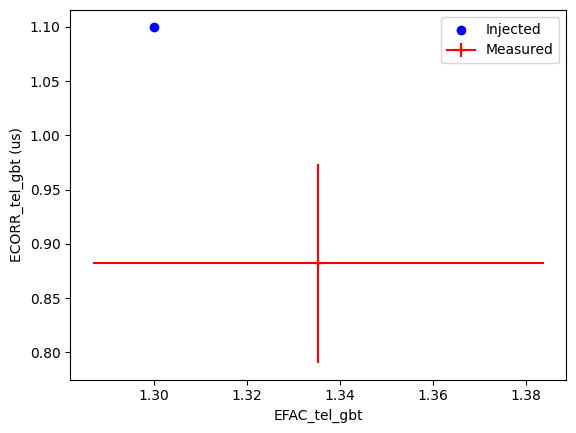
# Let us plot the injected and measured noise parameters together to
# compare them.
plt.scatter(m.EFAC1.value, m.ECORR1.value, label="Injected", marker="o", color="blue")
plt.errorbar(
    ftr.model.EFAC1.value,
    ftr.model.ECORR1.value,
    xerr=ftr.model.EFAC1.uncertainty_value,
    yerr=ftr.model.ECORR1.uncertainty_value,
    marker="+",
    label="Measured",
    color="red",
)
plt.xlabel("EFAC_tel_gbt")
plt.ylabel("ECORR_tel_gbt (us)")
plt.legend()
plt.show()