This Jupyter notebook can be downloaded from rednoise-fit-example.ipynb, or viewed as a python script at rednoise-fit-example.py.
Red noise, DM noise, and chromatic noise fitting examples
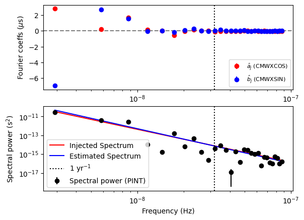
This notebook provides an example on how to fit for red noise and DM noise using PINT using simulated datasets.
We will use the PLRedNoise and PLDMNoise models to generate noise realizations (these models provide Fourier Gaussian process descriptions of achromatic red noise and DM noise respectively).
We will fit the generated datasets using the WaveX and DMWaveX models, which provide deterministic Fourier representations of achromatic red noise and DM noise respectively.
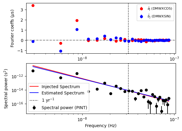
Finally, we will convert the WaveX/DMWaveX amplitudes into spectral parameters and compare them with the injected values.
[1]:
from pint import DMconst
from pint.models import get_model
from pint.simulation import make_fake_toas_uniform
from pint.logging import setup as setup_log
from pint.fitter import WLSFitter
from pint.utils import (
    cmwavex_setup,
    dmwavex_setup,
    find_optimal_nharms,
    plchromnoise_from_cmwavex,
    wavex_setup,
    plrednoise_from_wavex,
    pldmnoise_from_dmwavex,
)

from io import StringIO
import numpy as np
import astropy.units as u
from matplotlib import pyplot as plt
from copy import deepcopy

setup_log(level="WARNING")
[1]:
1
Red noise fitting
Simulation
The first step is to generate a simulated dataset for demonstration. Note that we are adding PHOFF as a free parameter. This is required for the fit to work properly.
[2]:
par_sim = """
    PSR           SIM3
    RAJ           05:00:00     1
    DECJ          15:00:00     1
    PEPOCH        55000
    F0            100          1
    F1            -1e-15       1
    PHOFF         0            1
    DM            15           1
    TNREDAMP      -13
    TNREDGAM      3.5
    TNREDC        30
    TZRMJD        55000
    TZRFRQ        1400
    TZRSITE       gbt
    UNITS         TDB
    EPHEM         DE440
    CLOCK         TT(BIPM2019)
"""

m = get_model(StringIO(par_sim))
[3]:
# Now generate the simulated TOAs.
ntoas = 2000
toaerrs = np.random.uniform(0.5, 2.0, ntoas) * u.us
freqs = np.linspace(500, 1500, 8) * u.MHz

t = make_fake_toas_uniform(
    startMJD=53001,
    endMJD=57001,
    ntoas=ntoas,
    model=m,
    freq=freqs,
    obs="gbt",
    error=toaerrs,
    add_noise=True,
    add_correlated_noise=True,
    name="fake",
    include_bipm=True,
    multi_freqs_in_epoch=True,
)
Optimal number of harmonics
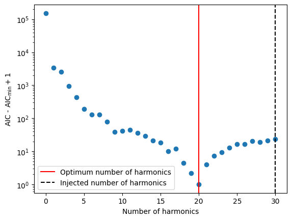
The optimal number of harmonics can be estimated by minimizing the Akaike Information Criterion (AIC). This is implemented in the pint.utils.find_optimal_nharms function.
[4]:
m1 = deepcopy(m)
m1.remove_component("PLRedNoise")

nharm_opt, d_aics = find_optimal_nharms(m1, t, "WaveX", 30)

print("Optimum no of harmonics = ", nharm_opt)
Optimum no of harmonics = 20
[5]:
print(np.argmin(d_aics))
20
[6]:
# The Y axis is plotted in log scale only for better visibility.
plt.scatter(list(range(len(d_aics))), d_aics + 1)
plt.axvline(nharm_opt, color="red", label="Optimum number of harmonics")
plt.axvline(
    int(m.TNREDC.value), color="black", ls="--", label="Injected number of harmonics"
)
plt.xlabel("Number of harmonics")
plt.ylabel("AIC - AIC$_\\min{} + 1$")
plt.legend()
plt.yscale("log")
# plt.savefig("sim3-aic.pdf")
[7]:
# Now create a new model with the optimum number of harmonics
m2 = deepcopy(m1)
Tspan = t.get_mjds().max() - t.get_mjds().min()
wavex_setup(m2, T_span=Tspan, n_freqs=nharm_opt, freeze_params=False)

ftr = WLSFitter(t, m2)
ftr.fit_toas(maxiter=10)
m2 = ftr.model

print(m2)
# Created: 2026-05-29T16:47:15.856298
# PINT_version: 1.1.5+106.g7d0f1d8
# User: docs
# Host: build-32906959-project-85767-nanograv-pint
# OS: Linux-7.0.0-1004-aws-x86_64-with-glibc2.35
# Python: 3.11.14 (main, Apr 27 2026, 17:28:30) [GCC 11.4.0]
# Format: pint
# read_time: 2026-05-29T16:46:26.414322
# allow_tcb: False
# convert_tcb: False
# allow_T2: False
PSR                                  SIM3
EPHEM                               DE440
CLOCK                        TT(BIPM2019)
UNITS                                 TDB
START              53000.9999999565507292
FINISH             56985.0000000463074421
DILATEFREQ                              N
DMDATA                                  N
NTOA                                 2000
CHI2                   1932.9733847762775
CHI2R                  0.9897457167313248
TRES                0.9723511668311587657
RAJ                      4:59:59.99983443 1 0.00011996322647783299
DECJ                    15:00:00.01398266 1 0.01189747098607950825
PMRA                                  0.0
PMDEC                                 0.0
PX                                    0.0
F0                   99.99999999999938162 1 5.646496443670277832e-13
F1              -1.000116217369479682e-15 1 1.8752305596513042508e-19
PEPOCH             55000.0000000000000000
PLANET_SHAPIRO                          N
DM                  14.999992604198467386 1 4.8123185704540527417e-06
WXEPOCH            55000.0000000000000000
WXFREQ_0001        0.00025100401605860213
WXSIN_0001        -2.5986777149872923e-06 1 6.335778086343505e-07
WXCOS_0001           1.85927145787171e-05 1 1.1325896628148997e-05
WXFREQ_0002         0.0005020080321172043
WXSIN_0002         -4.724987608709713e-07 1 3.1983788473345667e-07
WXCOS_0002        -3.4507239855610767e-06 1 2.875479687201616e-06
WXFREQ_0003         0.0007530120481758064
WXSIN_0003         1.2905972625327174e-06 1 2.233073484818582e-07
WXCOS_0003         1.0488082111780752e-06 1 1.3170460134996137e-06
WXFREQ_0004         0.0010040160642344085
WXSIN_0004         -3.120898850972374e-07 1 1.7820866045248314e-07
WXCOS_0004          5.957378547725346e-08 1 7.746610707140333e-07
WXFREQ_0005         0.0012550200802930107
WXSIN_0005         -6.644770460474371e-07 1 1.5547394000048096e-07
WXCOS_0005         3.6626892725825117e-07 1 5.281689826787485e-07
WXFREQ_0006         0.0015060240963516128
WXSIN_0006         1.6768354307992734e-07 1 1.449574249173535e-07
WXCOS_0006         -5.773109095790546e-07 1 4.0160372786387515e-07
WXFREQ_0007         0.0017570281124102147
WXSIN_0007        -1.7321372078896508e-07 1 1.4499070958612245e-07
WXCOS_0007         2.6697886355272974e-07 1 3.3577665972839424e-07
WXFREQ_0008          0.002008032128468817
WXSIN_0008         3.3936088911601745e-07 1 1.582813941891408e-07
WXCOS_0008        -3.2213948214835266e-07 1 3.1130148887159657e-07
WXFREQ_0009          0.002259036144527419
WXSIN_0009         3.7329183807931886e-08 1 1.9749948397496281e-07
WXCOS_0009          2.198854546708621e-07 1 3.3557248138591285e-07
WXFREQ_0010         0.0025100401605860213
WXSIN_0010         3.4169285443758274e-07 1 3.4289631374571267e-07
WXCOS_0010        -4.3843709704784186e-07 1 5.087730484772127e-07
WXFREQ_0011         0.0027610441766446232
WXSIN_0011          2.831275182533019e-06 1 2.834978478208333e-06
WXCOS_0011         -3.885049253681285e-06 1 3.6620303153178536e-06
WXFREQ_0012         0.0030120481927032256
WXSIN_0012        -1.5007782655886104e-07 1 2.0783518956644855e-07
WXCOS_0012          2.878756704595529e-07 1 2.3426471902616977e-07
WXFREQ_0013         0.0032630522087618275
WXSIN_0013         2.3078969429874475e-07 1 9.793389537627093e-08
WXCOS_0013         -1.230381081432747e-07 1 9.792719776028174e-08
WXFREQ_0014         0.0035140562248204294
WXSIN_0014         -7.264503635473853e-08 1 6.232871193848012e-08
WXCOS_0014         1.8660448126653455e-07 1 5.888312550119855e-08
WXFREQ_0015         0.0037650602408790318
WXSIN_0015           3.17205212117319e-08 1 4.810763514165204e-08
WXCOS_0015           -9.3277932358693e-08 1 4.4123721284301764e-08
WXFREQ_0016          0.004016064256937634
WXSIN_0016         1.0751753411366062e-08 1 4.0599869154848516e-08
WXCOS_0016         -9.809436483921216e-08 1 3.85654868109048e-08
WXFREQ_0017          0.004267068272996236
WXSIN_0017        -2.1304523734490086e-08 1 3.666008529811082e-08
WXCOS_0017         -5.378458640761075e-09 1 3.60956504699732e-08
WXFREQ_0018          0.004518072289054838
WXSIN_0018         -7.553734949551578e-08 1 3.4573463803850314e-08
WXCOS_0018         1.0380775574383492e-07 1 3.4452732015180066e-08
WXFREQ_0019           0.00476907630511344
WXSIN_0019          7.265723805877782e-08 1 3.3327682607436175e-08
WXCOS_0019         -4.937388670026597e-08 1 3.415815413849203e-08
WXFREQ_0020          0.005020080321172043
WXSIN_0020         -7.522097680418183e-08 1 3.31020285922585e-08
WXCOS_0020         -7.608737293515183e-09 1 3.372188911865298e-08
TZRMJD             55000.0000000000000000
TZRSITE                               gbt
TZRFRQ                             1400.0
PHOFF               0.0010407390065492624 1 0.000936551675915226
Estimating the spectral parameters from the WaveX fit.
[8]:
# Get the Fourier amplitudes and powers and their uncertainties.
idxs = np.array(m2.components["WaveX"].get_indices())
a = np.array([m2[f"WXSIN_{idx:04d}"].quantity.to_value("s") for idx in idxs])
da = np.array([m2[f"WXSIN_{idx:04d}"].uncertainty.to_value("s") for idx in idxs])
b = np.array([m2[f"WXCOS_{idx:04d}"].quantity.to_value("s") for idx in idxs])
db = np.array([m2[f"WXCOS_{idx:04d}"].uncertainty.to_value("s") for idx in idxs])
print(len(idxs))

P = (a**2 + b**2) / 2
dP = ((a * da) ** 2 + (b * db) ** 2) ** 0.5

f0 = (1 / Tspan).to_value(u.Hz)
fyr = (1 / u.year).to_value(u.Hz)
20
[9]:
# We can create a `PLRedNoise` model from the `WaveX` model.
# This will estimate the spectral parameters from the `WaveX`
# amplitudes.
m3 = plrednoise_from_wavex(m2)
print(m3)
# Created: 2026-05-29T16:47:15.905111
# PINT_version: 1.1.5+106.g7d0f1d8
# User: docs
# Host: build-32906959-project-85767-nanograv-pint
# OS: Linux-7.0.0-1004-aws-x86_64-with-glibc2.35
# Python: 3.11.14 (main, Apr 27 2026, 17:28:30) [GCC 11.4.0]
# Format: pint
# read_time: 2026-05-29T16:46:26.414322
# allow_tcb: False
# convert_tcb: False
# allow_T2: False
PSR                                  SIM3
EPHEM                               DE440
CLOCK                        TT(BIPM2019)
UNITS                                 TDB
START              53000.9999999565507292
FINISH             56985.0000000463074421
DILATEFREQ                              N
DMDATA                                  N
NTOA                                 2000
CHI2                   1932.9733847762775
CHI2R                  0.9897457167313248
TRES                0.9723511668311587657
RAJ                      4:59:59.99983443 1 0.00011996322647783299
DECJ                    15:00:00.01398266 1 0.01189747098607950825
PMRA                                  0.0
PMDEC                                 0.0
PX                                    0.0
F0                   99.99999999999938162 1 5.646496443670277832e-13
F1              -1.000116217369479682e-15 1 1.8752305596513042508e-19
PEPOCH             55000.0000000000000000
PLANET_SHAPIRO                          N
DM                  14.999992604198467386 1 4.8123185704540527417e-06
TZRMJD             55000.0000000000000000
TZRSITE                               gbt
TZRFRQ                             1400.0
PHOFF               0.0010407390065492624 1 0.000936551675915226
TNREDAMP              -12.860172222237331 0 0.0838358829549464
TNREDGAM                 2.78887852595373 0 0.46118958042177
TNREDC                                 20
[10]:
# Now let us plot the estimated spectrum with the injected
# spectrum.
plt.subplot(211)
plt.errorbar(
    idxs * f0,
    b * 1e6,
    db * 1e6,
    ls="",
    marker="o",
    label="$\\hat{a}_j$ (WXCOS)",
    color="red",
)
plt.errorbar(
    idxs * f0,
    a * 1e6,
    da * 1e6,
    ls="",
    marker="o",
    label="$\\hat{b}_j$ (WXSIN)",
    color="blue",
)
plt.axvline(fyr, color="black", ls="dotted")
plt.axhline(0, color="grey", ls="--")
plt.ylabel("Fourier coeffs ($\mu$s)")
plt.xscale("log")
plt.legend(fontsize=8)

plt.subplot(212)
plt.errorbar(
    idxs * f0, P, dP, ls="", marker="o", label="Spectral power (PINT)", color="k"
)
P_inj = m.components["PLRedNoise"].get_noise_weights(t)[::2][:nharm_opt]
plt.plot(idxs * f0, P_inj, label="Injected Spectrum", color="r")
P_est = m3.components["PLRedNoise"].get_noise_weights(t)[::2][:nharm_opt]
print(len(idxs), len(P_est))
plt.plot(idxs * f0, P_est, label="Estimated Spectrum", color="b")
plt.xscale("log")
plt.yscale("log")
plt.ylabel("Spectral power (s$^2$)")
plt.xlabel("Frequency (Hz)")
plt.axvline(fyr, color="black", ls="dotted", label="1 yr$^{-1}$")
plt.legend()
20 20
[10]:
<matplotlib.legend.Legend at 0x7a7953d15850>
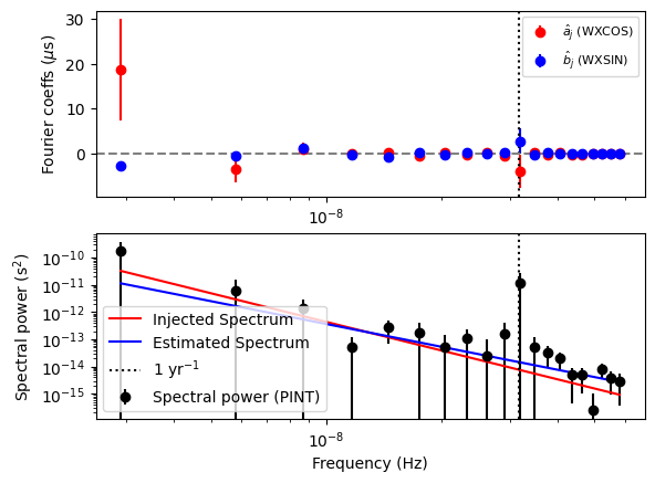
Note the outlier in the 1 year^-1 bin. This is caused by the covariance with RA and DEC, which introduce a delay with the same frequency.
DM noise fitting
Let us now do a similar kind of analysis for DM noise.
[11]:
par_sim = """
    PSR           SIM4
    RAJ           05:00:00     1
    DECJ          15:00:00     1
    PEPOCH        55000
    F0            100          1
    F1            -1e-15       1
    PHOFF         0            1
    DM            15           1
    TNDMAMP       -13
    TNDMGAM       3.5
    TNDMC         30
    TZRMJD        55000
    TZRFRQ        1400
    TZRSITE       gbt
    UNITS         TDB
    EPHEM         DE440
    CLOCK         TT(BIPM2019)
"""

m = get_model(StringIO(par_sim))
[12]:
# Generate the simulated TOAs.
ntoas = 2000
toaerrs = np.random.uniform(0.5, 2.0, ntoas) * u.us
freqs = np.linspace(500, 1500, 8) * u.MHz

t = make_fake_toas_uniform(
    startMJD=53001,
    endMJD=57001,
    ntoas=ntoas,
    model=m,
    freq=freqs,
    obs="gbt",
    error=toaerrs,
    add_noise=True,
    add_correlated_noise=True,
    name="fake",
    include_bipm=True,
    multi_freqs_in_epoch=True,
)
[13]:
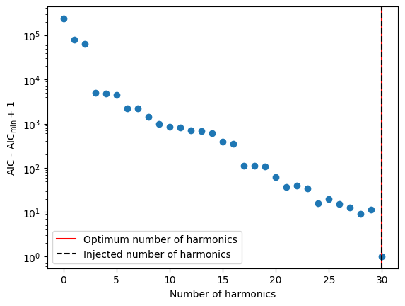
# Find the optimum number of harmonics by minimizing AIC.
m1 = deepcopy(m)
m1.remove_component("PLDMNoise")

m2 = deepcopy(m1)

nharm_opt, d_aics = find_optimal_nharms(m2, t, "DMWaveX", 30)
print("Optimum no of harmonics = ", nharm_opt)
Optimum no of harmonics = 30
[14]:
# The Y axis is plotted in log scale only for better visibility.
plt.scatter(list(range(len(d_aics))), d_aics + 1)
plt.axvline(nharm_opt, color="red", label="Optimum number of harmonics")
plt.axvline(
    int(m.TNDMC.value), color="black", ls="--", label="Injected number of harmonics"
)
plt.xlabel("Number of harmonics")
plt.ylabel("AIC - AIC$_\\min{} + 1$")
plt.legend()
plt.yscale("log")
# plt.savefig("sim3-aic.pdf")
[15]:
# Now create a new model with the optimum number of
# harmonics
m2 = deepcopy(m1)

Tspan = t.get_mjds().max() - t.get_mjds().min()
dmwavex_setup(m2, T_span=Tspan, n_freqs=nharm_opt, freeze_params=False)

ftr = WLSFitter(t, m2)
ftr.fit_toas(maxiter=10)
m2 = ftr.model

print(m2)
# Created: 2026-05-29T16:48:14.331971
# PINT_version: 1.1.5+106.g7d0f1d8
# User: docs
# Host: build-32906959-project-85767-nanograv-pint
# OS: Linux-7.0.0-1004-aws-x86_64-with-glibc2.35
# Python: 3.11.14 (main, Apr 27 2026, 17:28:30) [GCC 11.4.0]
# Format: pint
# read_time: 2026-05-29T16:47:16.615729
# allow_tcb: False
# convert_tcb: False
# allow_T2: False
PSR                                  SIM4
EPHEM                               DE440
CLOCK                        TT(BIPM2019)
UNITS                                 TDB
START              53000.9999999566237616
FINISH             56985.0000000459682407
DILATEFREQ                              N
DMDATA                                  N
NTOA                                 2000
CHI2                   1898.5737109406743
CHI2R                  0.9821902281120922
TRES                0.9948257184096412275
RAJ                      4:59:59.99999927 1 0.00000189756550630250
DECJ                    15:00:00.00031896 1 0.00016481477141845282
PMRA                                  0.0
PMDEC                                 0.0
PX                                    0.0
F0                   99.99999999999990025 1 3.6111685124766174305e-14
F1              -1.0000010072216736163e-15 1 8.3542934757783247666e-22
PEPOCH             55000.0000000000000000
PLANET_SHAPIRO                          N
DM                  15.000003792970505286 1 4.94926225308287409e-06
DMWXEPOCH          55000.0000000000000000
DMWXFREQ_0001       0.0002510040160586278
DMWXSIN_0001        -5.19829460711682e-05 1 6.016387589095863e-06
DMWXCOS_0001         0.001614496003940929 1 6.7097169465026494e-06
DMWXFREQ_0002       0.0005020080321172555
DMWXSIN_0002       -0.0004908640946712293 1 4.794866870160164e-06
DMWXCOS_0002       -0.0001416403171843871 1 4.499999841748996e-06
DMWXFREQ_0003       0.0007530120481758834
DMWXSIN_0003        0.0005013425500115456 1 4.4873917532548185e-06
DMWXCOS_0003        0.0009111836799463623 1 4.3993203728753266e-06
DMWXFREQ_0004        0.001004016064234511
DMWXSIN_0004         5.10268262626236e-05 1 4.488110073616618e-06
DMWXCOS_0004       -7.821053228976016e-06 1 4.285682953044387e-06
DMWXFREQ_0005        0.001255020080293139
DMWXSIN_0005        7.690939709111078e-05 1 4.431420767437971e-06
DMWXCOS_0005        5.071259104746735e-06 1 4.299856720988695e-06
DMWXFREQ_0006       0.0015060240963517667
DMWXSIN_0006       0.00019131100622559905 1 4.3600974024162435e-06
DMWXCOS_0006        9.008161725247661e-05 1 4.3522765995726275e-06
DMWXFREQ_0007       0.0017570281124103945
DMWXSIN_0007       2.4775121077730096e-05 1 4.482865193059918e-06
DMWXCOS_0007       2.7211486728034885e-05 1 4.2245630669669625e-06
DMWXFREQ_0008        0.002008032128469022
DMWXSIN_0008       0.00011894910780168976 1 4.388531259634993e-06
DMWXCOS_0008       -3.623848773972704e-05 1 4.326753865189494e-06
DMWXFREQ_0009         0.00225903614452765
DMWXSIN_0009        8.460472225123285e-05 1 4.34341789303768e-06
DMWXCOS_0009      -2.1124815498925768e-07 1 4.376557273421773e-06
DMWXFREQ_0010        0.002510040160586278
DMWXSIN_0010       -3.203897161712121e-05 1 4.408449102392102e-06
DMWXCOS_0010        4.062673797599414e-05 1 4.348766152187943e-06
DMWXFREQ_0011       0.0027610441766449056
DMWXSIN_0011      -3.5952412201794084e-05 1 6.837338670783943e-06
DMWXCOS_0011      -4.3124660311299944e-05 1 7.0674326179425735e-06
DMWXFREQ_0012       0.0030120481927035335
DMWXSIN_0012         5.06439403124638e-05 1 4.432805280334062e-06
DMWXCOS_0012      -1.6761728919114047e-05 1 4.27850031292624e-06
DMWXFREQ_0013       0.0032630522087621614
DMWXSIN_0013      -1.1254013097915179e-05 1 4.3381611765535665e-06
DMWXCOS_0013       1.0744429108022162e-05 1 4.340583894779777e-06
DMWXFREQ_0014        0.003514056224820789
DMWXSIN_0014      -2.4747702960537086e-05 1 4.31099217144167e-06
DMWXCOS_0014       2.5144532129452022e-05 1 4.341951695008588e-06
DMWXFREQ_0015        0.003765060240879417
DMWXSIN_0015      -4.9274661051405147e-05 1 4.353683212415028e-06
DMWXCOS_0015        3.481128018079075e-05 1 4.30360108582308e-06
DMWXFREQ_0016        0.004016064256938044
DMWXSIN_0016      -1.1392996285954889e-05 1 4.339128934208056e-06
DMWXCOS_0016       1.7971874510312684e-05 1 4.314193437688503e-06
DMWXFREQ_0017        0.004267068272996673
DMWXSIN_0017       2.1075685359667812e-05 1 4.317624977038542e-06
DMWXCOS_0017       -6.182015378494278e-05 1 4.328491973523769e-06
DMWXFREQ_0018          0.0045180722890553
DMWXSIN_0018        6.717344061977127e-06 1 4.2933962246984415e-06
DMWXCOS_0018       6.6846327124661176e-06 1 4.361956991072238e-06
DMWXFREQ_0019        0.004769076305113928
DMWXSIN_0019      -1.5761773031245934e-06 1 4.3516768297757305e-06
DMWXCOS_0019      -7.1920979799880424e-06 1 4.297604350478191e-06
DMWXFREQ_0020        0.005020080321172556
DMWXSIN_0020       -2.721096556889683e-05 1 4.391704522932104e-06
DMWXCOS_0020      -1.5303846587573006e-05 1 4.253200974822842e-06
DMWXFREQ_0021        0.005271084337231184
DMWXSIN_0021         8.53894207234787e-06 1 4.236723458446449e-06
DMWXCOS_0021      -1.9903572887633202e-05 1 4.39813167012964e-06
DMWXFREQ_0022        0.005522088353289811
DMWXSIN_0022         1.94970440748443e-06 1 4.432405631413965e-06
DMWXCOS_0022        3.871025727803045e-06 1 4.209148228293505e-06
DMWXFREQ_0023       0.0057730923693484395
DMWXSIN_0023       -3.325546721154002e-06 1 4.322963666649404e-06
DMWXCOS_0023      -1.3410967699982185e-05 1 4.325530939062148e-06
DMWXFREQ_0024        0.006024096385407067
DMWXSIN_0024         6.59534126334603e-06 1 4.40943615253564e-06
DMWXCOS_0024          1.8638003748487e-05 1 4.229734494287253e-06
DMWXFREQ_0025       0.0062751004014656945
DMWXSIN_0025      -1.2121386777277538e-06 1 4.291630379806682e-06
DMWXCOS_0025       1.3757435928347607e-06 1 4.341372771240231e-06
DMWXFREQ_0026        0.006526104417524323
DMWXSIN_0026       -5.888151778881874e-06 1 4.358100336611172e-06
DMWXCOS_0026        9.819340307314274e-06 1 4.26596188267779e-06
DMWXFREQ_0027         0.00677710843358295
DMWXSIN_0027       -7.850534537603138e-06 1 4.354104801452072e-06
DMWXCOS_0027       -7.305826725958442e-06 1 4.266176409696024e-06
DMWXFREQ_0028        0.007028112449641578
DMWXSIN_0028       -4.105988699763115e-06 1 4.33182821413844e-06
DMWXCOS_0028        1.190900426802579e-05 1 4.295518701901654e-06
DMWXFREQ_0029        0.007279116465700206
DMWXSIN_0029       -2.659441062472318e-06 1 4.297390358276559e-06
DMWXCOS_0029         5.09185852345841e-06 1 4.321691638348643e-06
DMWXFREQ_0030        0.007530120481758834
DMWXSIN_0030       1.1844607278539735e-05 1 4.355767690864851e-06
DMWXCOS_0030      -1.1500477702246456e-05 1 4.264648344391257e-06
TZRMJD             55000.0000000000000000
TZRSITE                               gbt
TZRFRQ                             1400.0
PHOFF               0.0005228618240355822 1 5.638302925253441e-06
Estimating the spectral parameters from the DMWaveX fit.
[16]:
# Get the Fourier amplitudes and powers and their uncertainties.
# Note that the `DMWaveX` amplitudes have the units of DM.
# We multiply them by a constant factor to convert them to dimensions
# of time so that they are consistent with `PLDMNoise`.
scale = DMconst / (1400 * u.MHz) ** 2

idxs = np.array(m2.components["DMWaveX"].get_indices())
a = np.array(
    [(scale * m2[f"DMWXSIN_{idx:04d}"].quantity).to_value("s") for idx in idxs]
)
da = np.array(
    [(scale * m2[f"DMWXSIN_{idx:04d}"].uncertainty).to_value("s") for idx in idxs]
)
b = np.array(
    [(scale * m2[f"DMWXCOS_{idx:04d}"].quantity).to_value("s") for idx in idxs]
)
db = np.array(
    [(scale * m2[f"DMWXCOS_{idx:04d}"].uncertainty).to_value("s") for idx in idxs]
)
print(len(idxs))

P = (a**2 + b**2) / 2
dP = ((a * da) ** 2 + (b * db) ** 2) ** 0.5

f0 = (1 / Tspan).to_value(u.Hz)
fyr = (1 / u.year).to_value(u.Hz)
30
[17]:
# We can create a `PLDMNoise` model from the `DMWaveX` model.
# This will estimate the spectral parameters from the `DMWaveX`
# amplitudes.
m3 = pldmnoise_from_dmwavex(m2)
print(m3)
# Created: 2026-05-29T16:48:14.392987
# PINT_version: 1.1.5+106.g7d0f1d8
# User: docs
# Host: build-32906959-project-85767-nanograv-pint
# OS: Linux-7.0.0-1004-aws-x86_64-with-glibc2.35
# Python: 3.11.14 (main, Apr 27 2026, 17:28:30) [GCC 11.4.0]
# Format: pint
# read_time: 2026-05-29T16:47:16.615729
# allow_tcb: False
# convert_tcb: False
# allow_T2: False
PSR                                  SIM4
EPHEM                               DE440
CLOCK                        TT(BIPM2019)
UNITS                                 TDB
START              53000.9999999566237616
FINISH             56985.0000000459682407
DILATEFREQ                              N
DMDATA                                  N
NTOA                                 2000
CHI2                   1898.5737109406743
CHI2R                  0.9821902281120922
TRES                0.9948257184096412275
RAJ                      4:59:59.99999927 1 0.00000189756550630250
DECJ                    15:00:00.00031896 1 0.00016481477141845282
PMRA                                  0.0
PMDEC                                 0.0
PX                                    0.0
F0                   99.99999999999990025 1 3.6111685124766174305e-14
F1              -1.0000010072216736163e-15 1 8.3542934757783247666e-22
PEPOCH             55000.0000000000000000
PLANET_SHAPIRO                          N
DM                  15.000003792970505286 1 4.94926225308287409e-06
TZRMJD             55000.0000000000000000
TZRSITE                               gbt
TZRFRQ                             1400.0
PHOFF               0.0005228618240355822 1 5.638302925253441e-06
TNDMAMP                 -12.9908309975989 0 0.041939680516696345
TNDMGAM                 3.342468255719136 0 0.25465418004392604
TNDMC                                  30
[18]:
# Now let us plot the estimated spectrum with the injected
# spectrum.
plt.subplot(211)
plt.errorbar(
    idxs * f0,
    b * 1e6,
    db * 1e6,
    ls="",
    marker="o",
    label="$\\hat{a}_j$ (DMWXCOS)",
    color="red",
)
plt.errorbar(
    idxs * f0,
    a * 1e6,
    da * 1e6,
    ls="",
    marker="o",
    label="$\\hat{b}_j$ (DMWXSIN)",
    color="blue",
)
plt.axvline(fyr, color="black", ls="dotted")
plt.axhline(0, color="grey", ls="--")
plt.ylabel("Fourier coeffs ($\mu$s)")
plt.xscale("log")
plt.legend(fontsize=8)

plt.subplot(212)
plt.errorbar(
    idxs * f0, P, dP, ls="", marker="o", label="Spectral power (PINT)", color="k"
)
P_inj = m.components["PLDMNoise"].get_noise_weights(t)[::2][:nharm_opt]
plt.plot(idxs * f0, P_inj, label="Injected Spectrum", color="r")
P_est = m3.components["PLDMNoise"].get_noise_weights(t)[::2][:nharm_opt]
print(len(idxs), len(P_est))
plt.plot(idxs * f0, P_est, label="Estimated Spectrum", color="b")
plt.xscale("log")
plt.yscale("log")
plt.ylabel("Spectral power (s$^2$)")
plt.xlabel("Frequency (Hz)")
plt.axvline(fyr, color="black", ls="dotted", label="1 yr$^{-1}$")
plt.legend()
30 30
[18]:
<matplotlib.legend.Legend at 0x7a7951159a10>
Chromatic noise fitting
Let us now do a similar kind of analysis for chromatic noise.
[19]:
par_sim = """
    PSR           SIM5
    RAJ           05:00:00     1
    DECJ          15:00:00     1
    PEPOCH        55000
    F0            100          1
    F1            -1e-15       1
    PHOFF         0            1
    DM            15
    CM            1.2          1
    TNCHROMIDX    3.5
    TNCHROMAMP    -13
    TNCHROMGAM    3.5
    TNCHROMC      30
    TZRMJD        55000
    TZRFRQ        1400
    TZRSITE       gbt
    UNITS         TDB
    EPHEM         DE440
    CLOCK         TT(BIPM2019)
"""

m = get_model(StringIO(par_sim))
[20]:
# Generate the simulated TOAs.
ntoas = 2000
toaerrs = np.random.uniform(0.5, 2.0, ntoas) * u.us
freqs = np.linspace(500, 1500, 8) * u.MHz

t = make_fake_toas_uniform(
    startMJD=53001,
    endMJD=57001,
    ntoas=ntoas,
    model=m,
    freq=freqs,
    obs="gbt",
    error=toaerrs,
    add_noise=True,
    add_correlated_noise=True,
    name="fake",
    include_bipm=True,
    multi_freqs_in_epoch=True,
)
[21]:
# Find the optimum number of harmonics by minimizing AIC.
m1 = deepcopy(m)
m1.remove_component("PLChromNoise")

m2 = deepcopy(m1)

nharm_opt = m.TNCHROMC.value
[22]:
# Now create a new model with the optimum number of
# harmonics
m2 = deepcopy(m1)

Tspan = t.get_mjds().max() - t.get_mjds().min()
cmwavex_setup(m2, T_span=Tspan, n_freqs=nharm_opt, freeze_params=False)

ftr = WLSFitter(t, m2)
ftr.fit_toas(maxiter=10)
m2 = ftr.model

print(m2)
# Created: 2026-05-29T16:48:24.311002
# PINT_version: 1.1.5+106.g7d0f1d8
# User: docs
# Host: build-32906959-project-85767-nanograv-pint
# OS: Linux-7.0.0-1004-aws-x86_64-with-glibc2.35
# Python: 3.11.14 (main, Apr 27 2026, 17:28:30) [GCC 11.4.0]
# Format: pint
# read_time: 2026-05-29T16:48:14.859679
# allow_tcb: False
# convert_tcb: False
# allow_T2: False
PSR                                  SIM5
EPHEM                               DE440
CLOCK                        TT(BIPM2019)
UNITS                                 TDB
START              53000.9999999566684376
FINISH             56985.0000000446357292
DILATEFREQ                              N
DMDATA                                  N
NTOA                                 2000
CHI2                   1966.6683080731748
CHI2R                  1.0174176451490817
TRES                1.0072077686915135882
RAJ                      4:59:59.99999813 1 0.00000145931064946389
DECJ                    15:00:00.00001053 1 0.00012441502473939636
PMRA                                  0.0
PMDEC                                 0.0
PX                                    0.0
F0                  99.999999999999992846 1 2.936025620379440699e-14
F1              -9.999994778613560655e-16 1 6.4957105998802578593e-22
PEPOCH             55000.0000000000000000
PLANET_SHAPIRO                          N
DM                                   15.0
CM                  1.0947326826560092591 1 0.051819808731836509985
TNCHROMIDX                            3.5
CMWXEPOCH          55000.0000000000000000
CMWXFREQ_0001       0.0002510040160587149
CMWXSIN_0001           -171.9117565208264 1 0.0677409321288027
CMWXCOS_0001            70.28307480831066 1 0.07242258390534091
CMWXFREQ_0002       0.0005020080321174298
CMWXSIN_0002            67.68132998787907 1 0.0593927836782618
CMWXCOS_0002             6.18001461558228 1 0.06109602602363355
CMWXFREQ_0003       0.0007530120481761447
CMWXSIN_0003            38.92624087234749 1 0.059249889758378714
CMWXCOS_0003           42.012545961695054 1 0.059369586537964175
CMWXFREQ_0004       0.0010040160642348596
CMWXSIN_0004          -0.2607274350560348 1 0.05909672029131714
CMWXCOS_0004           3.6897263537968925 1 0.05911082479762971
CMWXFREQ_0005       0.0012550200802935744
CMWXSIN_0005           1.2645277023622916 1 0.059803945579542835
CMWXCOS_0005           0.7267812349732367 1 0.057977077632847866
CMWXFREQ_0006       0.0015060240963522893
CMWXSIN_0006           -4.638449052633973 1 0.058729847566636864
CMWXCOS_0006          -13.030400199872652 1 0.058833394103674455
CMWXFREQ_0007       0.0017570281124110042
CMWXSIN_0007            2.787889374130071 1 0.0592002409836822
CMWXCOS_0007          -0.2061304353736251 1 0.0582273571072941
CMWXFREQ_0008        0.002008032128469719
CMWXSIN_0008             6.45925509523076 1 0.0588834057873422
CMWXCOS_0008            3.838746551834438 1 0.05828669820559719
CMWXFREQ_0009       0.0022590361445284338
CMWXSIN_0009          0.28207708734781367 1 0.05832340762721367
CMWXCOS_0009           1.3658302217904508 1 0.058845327899874664
CMWXFREQ_0010        0.002510040160587149
CMWXSIN_0010          -0.4714601431187238 1 0.058911117401499784
CMWXCOS_0010          0.23806034867430428 1 0.05852507170368701
CMWXFREQ_0011       0.0027610441766458636
CMWXSIN_0011          0.18201812006742563 1 0.07249026736481093
CMWXCOS_0011          -2.1668235554693642 1 0.07322123531747514
CMWXFREQ_0012       0.0030120481927045787
CMWXSIN_0012           3.2291644892542735 1 0.059233671115617004
CMWXCOS_0012         -0.24585336166126895 1 0.05779256977671985
CMWXFREQ_0013       0.0032630522087632933
CMWXSIN_0013           1.1163901556155458 1 0.05728253351466604
CMWXCOS_0013          -1.4407538756184903 1 0.05962178346337103
CMWXFREQ_0014       0.0035140562248220084
CMWXSIN_0014      -0.00030058391684485345 1 0.057179100682093156
CMWXCOS_0014         -0.12246186611857374 1 0.059631751006375015
CMWXFREQ_0015        0.003765060240880723
CMWXSIN_0015          0.41668354398832624 1 0.058736164971909414
CMWXCOS_0015          -1.4973906613514538 1 0.05821922836248626
CMWXFREQ_0016        0.004016064256939438
CMWXSIN_0016           0.4154875809678952 1 0.06048198746524693
CMWXCOS_0016        -0.060478728386444185 1 0.05624576540332162
CMWXFREQ_0017        0.004267068272998153
CMWXSIN_0017            1.879808075135482 1 0.05883045091625715
CMWXCOS_0017           0.4670439837779776 1 0.05798368513675296
CMWXFREQ_0018       0.0045180722890568676
CMWXSIN_0018           -1.430460810413343 1 0.05777899817612045
CMWXCOS_0018            1.124003947548139 1 0.05908023232226516
CMWXFREQ_0019        0.004769076305115583
CMWXSIN_0019          -0.6503689488509775 1 0.05803030759395253
CMWXCOS_0019           -1.070959960730329 1 0.05872777727991956
CMWXFREQ_0020        0.005020080321174298
CMWXSIN_0020         0.008310211601077422 1 0.05743328292561289
CMWXCOS_0020           1.1204627806460996 1 0.059136773590300507
CMWXFREQ_0021        0.005271084337233013
CMWXSIN_0021           0.5653885465014311 1 0.05735551906831187
CMWXCOS_0021          -1.1055438515892577 1 0.05917849398332885
CMWXFREQ_0022        0.005522088353291727
CMWXSIN_0022          -0.1482951395768682 1 0.0584458549102759
CMWXCOS_0022         -0.22716125920728913 1 0.0581023780737661
CMWXFREQ_0023        0.005773092369350442
CMWXSIN_0023         -0.37393405294539545 1 0.05722799117360123
CMWXCOS_0023           0.6716930844432477 1 0.05935140184912424
CMWXFREQ_0024        0.006024096385409157
CMWXSIN_0024          -0.6673373257013742 1 0.0588023600080758
CMWXCOS_0024         -0.32752304104609165 1 0.05780683054441555
CMWXFREQ_0025       0.0062751004014678724
CMWXSIN_0025         -0.09967251923417463 1 0.05897674020486762
CMWXCOS_0025         -0.38224302866201043 1 0.0578847436257752
CMWXFREQ_0026        0.006526104417526587
CMWXSIN_0026         -0.25699228404285757 1 0.057431982053168504
CMWXCOS_0026         -0.24585591774605106 1 0.059688198899298175
CMWXFREQ_0027        0.006777108433585302
CMWXSIN_0027          0.25142679290096925 1 0.05739736384795142
CMWXCOS_0027          -0.7633291678831668 1 0.059576708620168894
CMWXFREQ_0028        0.007028112449644017
CMWXSIN_0028          -0.5446896526160074 1 0.05851648340794401
CMWXCOS_0028         -0.43474841126226643 1 0.058505014988347814
CMWXFREQ_0029        0.007279116465702732
CMWXSIN_0029         0.005229514532230574 1 0.058089969105885465
CMWXCOS_0029          -0.3411158582287355 1 0.059005274867841295
CMWXFREQ_0030        0.007530120481761446
CMWXSIN_0030           0.4285675909276712 1 0.05876318267762235
CMWXCOS_0030         -0.13160284155238927 1 0.05830444706409294
TZRMJD             55000.0000000000000000
TZRSITE                               gbt
TZRFRQ                             1400.0
PHOFF              0.00044220744098781367 1 4.200594769474286e-06
Estimating the spectral parameters from the CMWaveX fit.
[23]:
# Get the Fourier amplitudes and powers and their uncertainties.
# Note that the `CMWaveX` amplitudes have the units of pc/cm^3/MHz^2.
# We multiply them by a constant factor to convert them to dimensions
# of time so that they are consistent with `PLChromNoise`.
scale = DMconst / 1400**m.TNCHROMIDX.value

idxs = np.array(m2.components["CMWaveX"].get_indices())
a = np.array(
    [(scale * m2[f"CMWXSIN_{idx:04d}"].quantity).to_value("s") for idx in idxs]
)
da = np.array(
    [(scale * m2[f"CMWXSIN_{idx:04d}"].uncertainty).to_value("s") for idx in idxs]
)
b = np.array(
    [(scale * m2[f"CMWXCOS_{idx:04d}"].quantity).to_value("s") for idx in idxs]
)
db = np.array(
    [(scale * m2[f"CMWXCOS_{idx:04d}"].uncertainty).to_value("s") for idx in idxs]
)
print(len(idxs))

P = (a**2 + b**2) / 2
dP = ((a * da) ** 2 + (b * db) ** 2) ** 0.5

f0 = (1 / Tspan).to_value(u.Hz)
fyr = (1 / u.year).to_value(u.Hz)
30
[24]:
# We can create a `PLChromNoise` model from the `CMWaveX` model.
# This will estimate the spectral parameters from the `CMWaveX`
# amplitudes.
m3 = plchromnoise_from_cmwavex(m2)
print(m3)
# Created: 2026-05-29T16:48:24.371492
# PINT_version: 1.1.5+106.g7d0f1d8
# User: docs
# Host: build-32906959-project-85767-nanograv-pint
# OS: Linux-7.0.0-1004-aws-x86_64-with-glibc2.35
# Python: 3.11.14 (main, Apr 27 2026, 17:28:30) [GCC 11.4.0]
# Format: pint
# read_time: 2026-05-29T16:48:14.859679
# allow_tcb: False
# convert_tcb: False
# allow_T2: False
PSR                                  SIM5
EPHEM                               DE440
CLOCK                        TT(BIPM2019)
UNITS                                 TDB
START              53000.9999999566684376
FINISH             56985.0000000446357292
DILATEFREQ                              N
DMDATA                                  N
NTOA                                 2000
CHI2                   1966.6683080731748
CHI2R                  1.0174176451490817
TRES                1.0072077686915135882
RAJ                      4:59:59.99999813 1 0.00000145931064946389
DECJ                    15:00:00.00001053 1 0.00012441502473939636
PMRA                                  0.0
PMDEC                                 0.0
PX                                    0.0
F0                  99.999999999999992846 1 2.936025620379440699e-14
F1              -9.999994778613560655e-16 1 6.4957105998802578593e-22
PEPOCH             55000.0000000000000000
PLANET_SHAPIRO                          N
DM                                   15.0
CM                  1.0947326826560092591 1 0.051819808731836509985
TNCHROMIDX                            3.5
TZRMJD             55000.0000000000000000
TZRSITE                               gbt
TZRFRQ                             1400.0
PHOFF              0.00044220744098781367 1 4.200594769474286e-06
TNCHROMAMP             -13.00920934509816 0 0.04015357685673689
TNCHROMGAM              3.672249253839617 0 0.21749920178312804
TNCHROMC                               30
[25]:
# Now let us plot the estimated spectrum with the injected
# spectrum.
plt.subplot(211)
plt.errorbar(
    idxs * f0,
    b * 1e6,
    db * 1e6,
    ls="",
    marker="o",
    label="$\\hat{a}_j$ (CMWXCOS)",
    color="red",
)
plt.errorbar(
    idxs * f0,
    a * 1e6,
    da * 1e6,
    ls="",
    marker="o",
    label="$\\hat{b}_j$ (CMWXSIN)",
    color="blue",
)
plt.axvline(fyr, color="black", ls="dotted")
plt.axhline(0, color="grey", ls="--")
plt.ylabel("Fourier coeffs ($\mu$s)")
plt.xscale("log")
plt.legend(fontsize=8)

plt.subplot(212)
plt.errorbar(
    idxs * f0, P, dP, ls="", marker="o", label="Spectral power (PINT)", color="k"
)
P_inj = m.components["PLChromNoise"].get_noise_weights(t)[::2]
plt.plot(idxs * f0, P_inj, label="Injected Spectrum", color="r")
P_est = m3.components["PLChromNoise"].get_noise_weights(t)[::2]
print(len(idxs), len(P_est))
plt.plot(idxs * f0, P_est, label="Estimated Spectrum", color="b")
plt.xscale("log")
plt.yscale("log")
plt.ylabel("Spectral power (s$^2$)")
plt.xlabel("Frequency (Hz)")
plt.axvline(fyr, color="black", ls="dotted", label="1 yr$^{-1}$")
plt.legend()
30 30
[25]:
<matplotlib.legend.Legend at 0x7a7951639010>
[ ]: